Q-Learning with Scalar Adjoint Matching: Cheaper Off-Policy RL for Flow Policies
A closed-form scalar adjoint removes the per-step vector–Jacobian products of adjoint matching, and a value penalty at the policy's own actions makes it work.
Adjoint matching propagates the critic’s gradient at the final action back to the flow steps that produced it. QAM and TRQAM integrate the lean adjoint ODE backward along the sampling chain, which takes a vector–Jacobian product \(J_i^\top\) through the policy at every flow step. SQAM instead scales the gradient at the final action by the flow time \(\tau\), with no vector–Jacobian product at any flow step.
Flow policies represent rich and multimodal action distributions. They have become a common policy class for offline and offline-to-online RL
Fine-tuning a flow policy against a learned critic is not trivial, because the policy generates its action over many flow steps
Adjoint matching
This post introduces Q-learning with Scalar Adjoint Matching (SQAM), which removes these per-step vector–Jacobian products. It rests on two findings. First, the velocity Jacobian of a pretrained flow policy is nearly diagonal, which gives a closed-form scalar adjoint. Second, under the scalar adjoint, controlling the critic at the policy’s own actions matters most, which motivates a value penalty at those actions.
Adjoint matching and its cost
A flow policy generates its action over many flow steps, and the critic only tells us how good the final action is. To improve the policy, each intermediate step also needs to know in which direction to push its state so that the final action gets a higher value.
Adjoint matching computes this direction for every step. Starting from the critic’s gradient at the final action, it passes that gradient back through the chain one step at a time by integrating the lean adjoint ODE,
\[d\tilde{a}_\tau = -\tilde{a}_\tau^\top \nabla_{X_\tau}\!\left(2 v^{\text{base}}(X_\tau, \tau) - \frac{1}{\tau} X_\tau\right) d\tau, \qquad \tilde{a}_1 = -\nabla_{X_1} Q^\pi(s, X_1).\]It then trains the fine-tuned velocity \(v_\theta^{\text{ft}}\) to match the gradient that this ODE delivers to each step,
\[\mathcal{L}_{\text{Adj-Match}}(\theta) = \mathbb{E}\!\left[\sum_\tau \left\| \frac{2}{\sigma(\tau)}\big(v_\theta^{\text{ft}}(X_\tau, \tau) - v^{\text{base}}(X_\tau, \tau)\big) + \sigma(\tau)\, \tilde{a}_\tau \right\|^2\right],\]where \(\sigma(\tau)\) is the noise schedule of the sampler. TRQAM
The lean adjoint ODE avoids backpropagation through time, but each step still multiplies the adjoint by the velocity Jacobian \(\nabla_{X_\tau} v^{\text{base}}(X_\tau, \tau)\). This is a vector–Jacobian product (VJP) through the policy network, repeated at every flow step. As pretrained flow policies grow into large vision-language-action models
The velocity Jacobian is nearly diagonal
Can we preserve this propagation without a policy VJP at every flow step? Our starting point is an empirical observation. The batch-averaged velocity Jacobian \(J_\tau := \nabla_{X_\tau} v^{\text{base}}(X_\tau, \tau)\) of a pretrained flow policy concentrates on its diagonal.
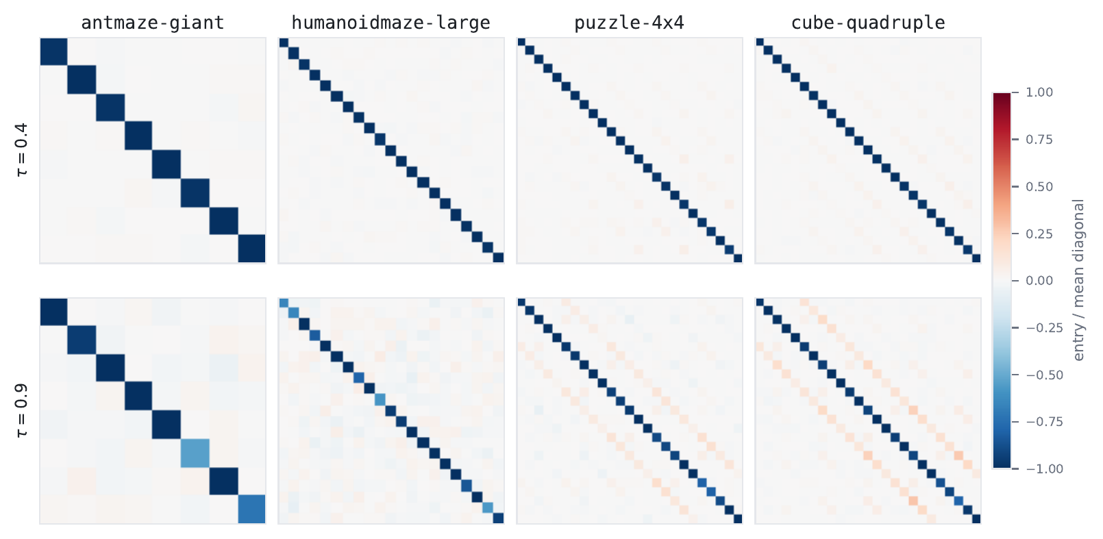
Velocity Jacobian of the pretrained flow on four OGBench domains at two flow times, averaged over a batch of states and normalized per panel by the mean diagonal. The batch-averaged Jacobian is dominated by its diagonal. The paper shows all ten domains.
Following the isotropic approximation of the posterior covariance in Peng et al.
Proposition 1 (the lean adjoint ODE under an isotropic velocity Jacobian). Assume \(J_\tau = c_\tau I\) for a scalar \(c_\tau\). Then the lean adjoint ODE admits the closed-form solution
\[\tilde{a}_\tau = -\,\tau \exp\!\Big(2\!\int_\tau^1 c_s\, ds\Big)\, \nabla_{X_1} Q^\pi(s, X_1),\]which points along the negative of the critic’s action gradient at the final action at every flow time \(\tau > 0\).
The proof is short. With \(J_\tau = c_\tau I\), the Jacobian term in the ODE becomes \(\big(\tfrac{1}{\tau} - 2c_\tau\big) I\), so every coordinate is scaled by the same factor. Integrating from \(\tau\) to \(1\) and applying the terminal condition gives the result.
The scalar adjoint
At every flow time, the closed-form solution is a scalar multiple of the critic’s action gradient at the final action. Estimating \(c_\tau\) would reintroduce the Jacobian we set out to avoid, so we drop the exponential factor and keep only
\[\hat{a}_\tau = -\tau\, \nabla_{X_1} Q^\pi(s, X_1), \qquad \forall \tau \in [0, 1].\]We call this the scalar adjoint. The exponential factor only rescales the closed-form solution, and dropping it is justified empirically below. The scalar adjoint needs a single critic gradient at the sampled action \(X_1\) and no VJP through the policy at any flow step.
SQAM keeps the adjoint matching loss above and simply replaces the exact adjoint \(\tilde{a}_\tau\) in its target with \(\hat{a}_\tau\). The path-space trust region of TRQAM can therefore be used or left out. We use it by default for stable training.
Regularizing the critic at the policy’s own actions
The scalar adjoint alone does not work well, especially on the manipulation domains. The exact adjoint passes \(\nabla_{X_1} Q^\pi(s, X_1)\) through the velocity Jacobian at every flow step, so it does not use this gradient as directly as the scalar adjoint does. The scalar adjoint update therefore depends directly on the critic’s gradient at the policy-generated action, and we hypothesize that its failure comes from critic errors at that action.
To address this, we add a value penalty on the critic at the actions the current policy generates, relative to the value at the dataset action,
\[\mathcal{L}_{\text{critic}} \mathrel{+}= c \cdot \big(Q^\pi(s, \operatorname{sg}(a_\pi)) - Q^\pi(s, a_{\text{data}})\big).\]The penalty acts at the policy-generated action \(a_\pi\), which is also the action whose critic gradient drives the scalar adjoint update. It therefore controls the critic exactly where the policy update uses it. Unlike CQL
Common forms of critic regularization act elsewhere. In-sample maximization
Require: vbase, Qπφ, KL budget εKL, training steps N
1:  vftθ ← vbase
2:  for n = 0, …, N−1 do
3:    Sample a trajectory X0, …, X1 by vftθ
4:    Xτ ← the states of that trajectory
5:    Solve the lean adjoint ODE for ãτ
6:    Update θ by the Adjoint Matching loss
7:    TD update of Qπφ
8:    Dual update of λn for trust region
9:  end for
Require: vbase, Qπφ, KL budget εKL, training steps N
1:  vftθ ← vbase
2:  for n = 0, …, N−1 do
3:    Sample the endpoint X1 by vftθ
4:    Xτ ← (1−τ) ε + τ X1,  ε ~ N(0, I)
5:    âτ ← −τ ∇X1Qπ(s, X1)
6:    Update θ by the Adjoint Matching loss
7:    TD update of Qπφ + value penalty
8:    Dual update of λn for trust region
9:  end for
Simplified versions of the TRQAM and SQAM algorithms. The parts SQAM changes are marked in blue. The full algorithm is in the appendix of the paper.
Results
We evaluate SQAM on the 50 OGBench
The gains of SQAM concentrate on the four hardest domains, where every prior method struggles. In each of them, TRQAM is the strongest baseline, and SQAM adds 18 to 35 percentage points of offline success on top of it. The largest gap is on cube-quadruple, where the strongest baseline reaches 19% and SQAM reaches 54%. These gains hold through the online phase as well.
Offline success rate (%) at 1M training steps on the four hardest OGBench domains (8 seeds, 5 tasks per domain). TRQAM is the strongest baseline on each of these domains.
View all 10 domain averages and methods
| Method | al | ag | hm | hl | scene | p33 | p44 | c2 | c3 | c4 | all | |
|---|---|---|---|---|---|---|---|---|---|---|---|---|
| 5 tasks | 5 tasks | 5 tasks | 5 tasks | 5 tasks | 5 tasks | 5 tasks | 5 tasks | 5 tasks | 5 tasks | 50 tasks | ||
| Backprop | FQL | 38±9 | 2±6 | 74±5 | 2±1 | 70±5 | 25±10 | 9±7 | 44±4 | 7±5 | 9±5 | 28 |
| Guidance | CGQL-L | 48±7 | 7±5 | 57±2 | 6±3 | 58±1 | 0±0 | 0±0 | 55±2 | 0±1 | 1±1 | 23 |
| Post Processing | DSRL | 53±2 | 1±1 | 53±10 | 1±1 | 80±0 | 100±0 | 61±8 | 72±4 | 34±6 | 9±3 | 46 |
| IFQL | 29±8 | 12±3 | 93±2 | 30±7 | 36±1 | 64±4 | 42±4 | 9±2 | 24±7 | 6±3 | 35 | |
| Adjoint Matching | QAM | 62±9 | 29±4 | 64±7 | 4±3 | 64±4 | 15±3 | 1±1 | 71±2 | 19±6 | 18±3 | 35 |
| QAM-E | 86±3 | 6±8 | 60±6 | 4±5 | 63±6 | 89±4 | 54±8 | 71±3 | 11±4 | 9±3 | 45 | |
| TRQAM | 89±4 | 41±4 | 84±3 | 36±4 | 79±1 | 100±0 | 99±1 | 81±3 | 50±5 | 19±5 | 68 | |
| Ours | SQAM | 91±3 | 62±4 | 94±2 | 54±5 | 79±0 | 100±0 | 85±6 | 58±3 | 72±4 | 54±5 | 75 |
Offline RL on 50 OGBench tasks at 1M training steps (8 seeds). Mean success rate (%) with ±1 standard deviation. Domain abbreviations are al = antmaze-large, ag = antmaze-giant, hm = humanoidmaze-medium, hl = humanoidmaze-large, p33 = puzzle-3x3, p44 = puzzle-4x4, c2 = cube-double, c3 = cube-triple, and c4 = cube-quadruple. Gray cells mark the best baseline per column, and SQAM is shown in blue.
Why does the scalar adjoint work?
The scalar adjoint is an approximation, yet it preserves the two properties the update relies on. To see this, we compute both adjoints on the same rollout states.

Exact and scalar adjoints computed on the same rollout states. Left, the norm of each adjoint relative to \(\|\nabla_a Q\|\), where the scalar adjoint is the dotted line \(\tau\). Right, the angle between the two adjoints. Three seeds per domain at 0.3M steps, without the value penalty.
- Similar contraction. Both adjoints contract in the same way as the flow time approaches zero. The regression target of the adjoint matching loss therefore has a similar magnitude at each flow step under either adjoint.
- Positive alignment. The scalar adjoint stays positively aligned with the exact adjoint at every flow time.
These two properties allow the scalar adjoint to stand in for the exact adjoint, but they do not make the two identical. The angle between them is larger on the two manipulation domains than on the two locomotion domains, and these are exactly the domains where the scalar adjoint alone underperforms. Since the scalar adjoint relies directly on the critic’s gradient, this correspondence led us to examine the role of the value learning scheme.
Which value learning scheme works?
We compare the value penalty with three alternatives. The first is an in-sample critic in the style of IQL

Value learning schemes compared on the two domains where the scalar adjoint alone fails. Each scheme is shown at its best coefficient on the grid we swept. Eight seeds per curve, and bands are one standard deviation.
The value penalty works best on both domains, while the in-sample critic and ReBRAC stay close to the scalar adjoint without regularization. This follows from where each scheme acts. The in-sample critic is trained only on dataset actions, so it never evaluates the critic at \(a_\pi\). ReBRAC constrains the distance between \(a_\pi\) and \(a_{\text{data}}\), which controls the action itself rather than the value the critic assigns to it. Only the value penalty acts on the critic’s value at \(a_\pi\).
The gradient-norm penalty also improves over the unregularized critic, most clearly on cube-quadruple. This is consistent with its close relation to the value penalty. A first-order expansion of the value penalty around \(a_\pi\) gives
so the two penalties are linked through the critic’s gradient at \(a_\pi\).
If this explanation holds, the value penalty should help the exact adjoint less, since the exact adjoint passes the critic’s gradient through the velocity Jacobian at every flow step. Applying the value penalty to TRQAM confirms this. It improves TRQAM as well, but far less than it improves SQAM.
Ablations
Value penalty coefficient \(c\). On the two cube manipulation tasks, the success rate rises sharply as \(c\) grows, while on the two locomotion tasks the gains are small. The value penalty therefore matters mainly on the domains where the scalar adjoint alone underperforms. We use \(c = 0.3\) on every domain except cube-double, where the penalty is off.

Sweep over the value penalty coefficient \(c\) on four of the ten swept domains. Eight seeds per curve, and bands are one standard deviation.
KL budget \(\varepsilon_{\text{KL}}\). The budget sets how far the fine-tuned policy may deviate from the pretrained one. On most domains, performance stays flat or decreases steadily as the budget widens, so the budget affects performance predictably and a small budget is a reliable default. The exception is puzzle-4x4, which prefers a larger budget, consistent with its larger state space.

Sweep over the KL budget \(\varepsilon_{\text{KL}}\) on four of the ten swept domains. Eight seeds per curve, and bands are one standard deviation.
Scaling to a pretrained vision-language-action policy
To test whether SQAM extends to large pretrained policies, we fine-tune RLDX-1

The three real-world manipulation tasks. From top to bottom, flipping a plastic bag, placing a straw in a cup, and placing fruit in a pot and closing the lid.
| Method | Flip plastic bag | Place the straw | Put the fruit and close the lid |
|---|---|---|---|
| SFT | 15/30 | 7/30 | 4/30 |
| EXPO-FT (offline) | 8/30 | 0/30 | 5/30 |
| EXPO-FT (offline-to-online) | 15/30 | 0/30 | 3/30 |
| SQAM (offline) | 20/30 | 13/30 | 8/30 |
| SQAM (offline-to-online) | 25/30 | 15/30 | 13/30 |
Success on three real-robot manipulation tasks, counted over 30 held-out episodes per task. The offline rows evaluate the checkpoint after 15K offline steps, and the offline-to-online rows the checkpoint after a further 10K online steps.
SQAM improves over SFT on all three tasks, whereas EXPO-FT does not appear to work well in this setting. SQAM updates the flow policy directly. EXPO-FT instead trains a residual edit policy, which must be learned from scratch and cannot directly exploit the expressiveness of the pretrained flow policy. We conjecture that these two differences account for the gap.
The videos below compare the two methods after offline-to-online fine-tuning, played at 2x speed.
Compute
Removing the per-step VJPs is what makes SQAM cheaper. We compare the wall-clock time of one SQAM update with that of the same update using the exact adjoint.

Wall-clock time of one update with the exact and the scalar adjoint. Left, actor width, with the critic fixed at 256×4. Right, number of flow steps. Percentages give the extra time of the exact adjoint.
When we widen the actor with the critic fixed, the exact adjoint remains about half again as slow at every width, so the saving persists on larger policies. As the number of flow steps increases, the gap grows, since the cost of the exact adjoint grows with the number of VJPs while the rest of the update does not.
Conclusion
SQAM fine-tunes flow policies with off-policy RL without a vector–Jacobian product through the policy. Motivated by the diagonal structure of the batch-averaged velocity Jacobian, it replaces the exact adjoint with a closed-form scalar adjoint and pairs it with a value penalty at the policy-generated actions. SQAM improves most on the four hardest OGBench domains and extends to a vision-language-action policy on a real robot.
Our results also suggest a broader point. A rough approximation of the adjoint suffices, while the value learning scheme largely determines how well it performs. The bottleneck of off-policy RL with flow policies may therefore lie less in the policy update than in the critic. We hope this encourages further work on value learning for flow policies.
BibTeX
@article{dong2026sqam,
    author  = {Yonghoon Dong and Minsung Yoon and Jaehyuk Kim and Jungwoo Park and Changyeon Kim and Jinwoo Shin},
    title   = {Q-Learning with Scalar Adjoint Matching},
    journal = {arXiv preprint arXiv:ARXIV_ID},
    year    = {2026}
}