Trust Region Q Adjoint Matching: Stable Off-Policy RL for Flow Policies
A new stable off-policy fine-tuning algorithm for pretrained flow-based policies, combining trust-region principles with stochastic optimal control.
A pretrained flow policy is a useful prior, but naive critic-guided fine-tuning (e.g., QAM, QAM-E) suffers from destructive drift. TRQAM internalizes a trust-region parameter \(\lambda\) inside the SOC sampling process and adapts it via dual descent.
Large pretrained flow-matching policies have rapidly become the dominant paradigm for robotics foundation models, with a growing family of vision-language-action (VLA) models
The natural next step is to fine-tune them with reinforcement learning, taking that pretrained prior and pushing it further with interaction data on the target task.
On a real robot, that fine-tuning has to be off-policy. Data collection is slow and expensive, every rollout takes wall-clock time, and exploratory actions can be physically dangerous. We cannot afford to throw away transitions after one update, so every transition we collect lives in a replay buffer and gets reused.
Off-policy RL on a flow policy, however, is structurally harder than off-policy RL on a more standard policy (e.g., a Gaussian or deterministic policy). The reason has to do with how a flow policy actually generates its actions.
What makes off-policy RL on flow policies difficult
A flow policy \(\pi_\theta(a \mid s)\) does not predict an action in one shot. It learns a velocity field \(v_\theta(X_\tau, \tau; s)\) that transports Gaussian noise to the action distribution, and samples an action by integrating the resulting ODE.
\[dX_\tau = v_\theta(X_\tau, \tau; s)\, d\tau, \quad X_0 \sim \mathcal{N}(0, I), \quad X_1 \sim \pi_\theta(\cdot \mid s).\]The reason for choosing a flow policy over a simpler parametric family is expressivity. A single Gaussian policy captures only one mode of action, whereas a flow policy captures rich multi-modal distributions
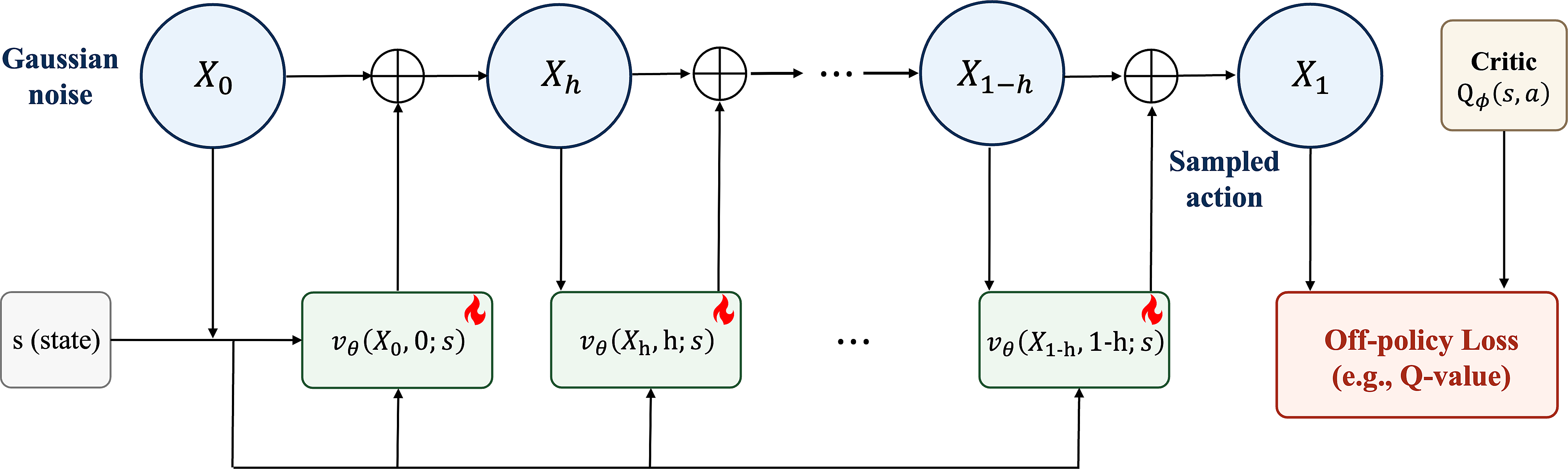
A flow policy produces an action by iteratively applying the velocity network from Gaussian noise. Naive off-policy fine-tuning backpropagates the terminal critic-guided loss through all sampling steps, making optimization prone to instability. (Figure style motivated by SAC Flow
That chain of denoising steps, however, is what makes off-policy RL on a flow policy structurally difficult. The figure above shows why. Modern off-policy RL is essentially Q-learning style actor-critic. It trains a critic $Q^\pi$ with a temporal-difference (TD) objective and improves the policy by following $\nabla_\theta Q^\pi$. For a Gaussian policy, that gradient is a single hop from action to parameters. For a flow policy, however, the critic’s signal has to travel all the way back from $X_1$ through every $v_\theta$ block in the figure to reach the policy parameters. This is exactly the same problem as backpropagation-through-time (BPTT) in RNNs
Existing workarounds and their trade-offs
Several strategies have appeared in the flow-policy RL literature to address backpropagation through the sampling chain. Each is principled, and each gives something up.
- One-step distillation (FQL
). Distill the multi-step flow policy into a one-step policy, then run Q-learning on top. - Pro: removes the chain entirely, and the resulting one-step policy is directly trainable with standard off-policy actor-critic.
- Con: the one-step policy has no built-in exploration mechanism for online fine-tuning.
- Noise-space RL (DSRL
). Freeze the flow policy and run RL in noise space, learning to sample the optimal noise $X_0$ that generates high-reward actions. - Pro: bypasses BPTT cleanly without touching the flow policy at all, and the multi-step structure is preserved as-is.
- Con: the policy’s action distribution is constrained to whatever the frozen pretrained flow policy can already produce. If the optimal action is not in its support, no choice of $X_0$ will recover it.
- Residual RL
. Freeze the flow policy and learn an additive residual $\Delta a$ at the action level. - Pro: simple to plug on top of any pretrained flow policy, and the residual is a small, easy-to-train head.
- Con: operates purely at the action-space level, ignoring the multi-step generative process that produced the action. The residual can shift the final output but cannot reshape the underlying generative dynamics.
- Architectural reparameterization (SAC Flow
). Reparameterize the velocity network into a stable sequence-model form, either a GRU-style recurrence or a specific attention-based structure, so that BPTT through the denoising chain is stable by design. - Pro: preserves the multi-step structure and allows the velocity field itself to be fine-tuned end-to-end.
- Con: forces the velocity network into one of these specific structural forms. Existing pretrained flow policies (e.g., the VLAs cited above) generally do not match them and cannot be reused as-is.
Each line of work buys around BPTT by giving something up, namely sacrificing exploration (FQL), restricting the search to noise space (DSRL), correcting only at the action level (residual), or constraining the model architecture (SAC Flow).
A more fundamental issue cuts across all four. None of these methods comes with any guarantee of converging to the optimal tilted distribution \(\pi^*_Q(a \mid s) \propto \pi_{\text{base}}(a \mid s)\, \exp\!\big(Q(s, a)\big),\) which is the policy that off-policy RL is implicitly trying to reach.
Addressing this gap calls for a framework that operates on the multi-step sampling dynamics directly without BPTT or architectural modifications to the velocity field, and that converges to the optimal tilted distribution.
That is exactly what stochastic optimal control (SOC) offers.
Q-learning with Adjoint Matching (QAM) and its hidden weakness
A recent line of work bypasses BPTT entirely by recasting policy improvement as a stochastic optimal control (SOC) problem guided by a learned critic
The idea is this. SOC steers the pretrained flow policy’s sampling process with a learned control \(u\) toward actions with low terminal cost. Training the flow model directly would require backpropagating through the multi-step sampling chain, which is costly and unstable, much like BPTT in RNNs. Adjoint Matching
Now let’s make this precise. A flow policy is originally a deterministic ODE, but SOC needs stochastic dynamics, so we first rewrite the ODE as an equivalent SDE that produces the same marginal distribution of \(X_\tau\) at every timestep \(\tau\), including the same terminal \(X_1 \sim \pi_{\text{base}}\) (the equivalence in distribution follows from the Fokker–Planck equation)
Here \(b(X_\tau, \tau)\) is the drift, the deterministic component that sets the overall direction in which the trajectory is pushed toward actions. The diffusion coefficient \(\sigma(\tau)\) is the stochastic counterpart, controlling how much noise the Brownian motion \(B_\tau\) injects into the trajectory.
SOC then adds the control \(u(X_\tau, \tau)\) on top of the drift, giving the controlled SDE, which describes the sampling dynamics once the control \(u\) is applied.
\[dX_\tau = \big[b(X_\tau, \tau) + \sigma(\tau)\, u(X_\tau, \tau)\big]\, d\tau + \sigma(\tau)\, dB_\tau.\]The added term \(\sigma(\tau)\, u(X_\tau, \tau)\) is what steers each step of the sampling process away from the pretrained trajectory. The base SDE generates the pretrained policy \(\pi_{\text{base}}\). The control \(u\) modifies this process, and its magnitude determines how far the resulting policy moves from \(\pi_{\text{base}}\).
Given a terminal cost \(g\) on the final action, SOC seeks the control \(u\) by optimizing
\[\min_u\;\mathbb{E}\!\left[\, \frac{1}{2}\!\int_0^1 \|u(X_\tau, \tau)\|^2 \, d\tau \;+\; g(X_1) \,\right] \quad \text{subject to the controlled SDE above,}\]where \(g(X_1)\) is called the terminal cost on the final action and \(\tfrac{1}{2}\!\int_0^1 \|u(X_\tau, \tau)\|^2 d\tau\) is called the quadratic cost on the control. The terminal cost encourages the trajectory to land at final actions \(X_1\) where \(g\) is small, and the quadratic cost penalizes the magnitude of \(u\). As we will see later, this quadratic cost is also what controls how far the sampling process deviates from the pretrained one, although the connection is not immediately apparent from the equation. The optimum is the smallest control magnitude that still achieves low terminal cost.
Which SDE should we use? The base SDE is not unique, since many diffusion coefficients give the same marginals once the drift is adjusted. Adjoint Matching
The schedule matters because under it, the initial noise \(X_0\) is independent of the final action \(X_1\). As a result, the optimum of the SOC objective exponentially tilts \(\pi_{\text{base}}\) toward low terminal cost,
\[\pi^*(a \mid s) \;\propto\; \pi_{\text{base}}(a \mid s)\, e^{-g(a)}.\]This is exactly the optimal tilted distribution from the previous section, once the terminal cost is set to the negative critic.
Q-learning with Adjoint Matching (QAM)
QAM solves this SOC problem with Adjoint Matching in two steps. First, it propagates the critic gradient at the final action back along the sampling trajectory. This gives the adjoint \(\tilde{a}_\tau\), obtained by integrating the following lean adjoint ODE backward in time, where the term in parentheses is the base drift \(b\) of the base SDE.
\[\tilde{a}_{\tau-h} = \tilde{a}_\tau + h\,\tilde{a}_\tau^\top \nabla_x\!\left(2 v^{\text{base}}(X_\tau, \tau) - \frac{1}{\tau}X_\tau\right), \quad \tilde{a}_1 = -\nabla_{x_1} Q^\pi(s, X_1).\]The terminal condition \(\tilde{a}_1 = -\nabla_{x_1} Q^\pi(s, X_1)\) is the negative critic gradient at the final action \(X_1\). The lean adjoint ODE then propagates this signal backward in time, giving \(\tilde{a}_\tau\) at each intermediate \(\tau\). This is the action-level cost signal, transported back to time \(\tau\). Crucially, \(\tilde{a}_\tau\) depends only on the pretrained \(v^{\text{base}}\) and the sampled trajectory, so it is \(\theta\)-independent.
Second, with \(\tilde{a}_\tau\) in hand, the fine-tuned velocity field \(v_\theta^{\text{ft}}\) is then trained by minimizing the adjoint matching loss.
\[\mathcal{L}_{\text{Adj-Match}}(\theta) = \sum_\tau \left\| \tfrac{2}{\sigma(\tau)}\big(v_\theta^{\text{ft}}(X_\tau, \tau) - v^{\text{base}}(X_\tau, \tau)\big) + \sigma(\tau)\, \tilde{a}_\tau \right\|^2,\]where \(v_\theta^{\text{ft}}\)’s deviation from the pretrained \(v^{\text{base}}\) parameterizes the control \(u\). The loss is minimized when this deviation aligns with the transported signal \(\tilde{a}_\tau\) at every timestep. Taking \(\nabla_\theta \mathcal{L}_{\text{Adj-Match}}\) only differentiates through \(v_\theta^{\text{ft}}\) at each \(\tau\) individually, never through the multi-step forward chain. This is what makes the BPTT problem disappear (for the full derivation and further details, we refer to the original Adjoint Matching paper
In this way, QAM injects the critic’s signal directly into every step of the multi-step generative process, making the sampling process itself critic-aware. The same paper also introduces a variant, QAM-E, which takes a QAM-trained policy and learns an additional residual RL correction at the action level on top of it.
So far so good. But both QAM and QAM-E inherit a more subtle problem, namely critic-induced instability.
In off-policy RL, the learned critic \(Q^\pi\) is inevitably imperfect. TD bootstrapping compounds approximation errors and tends to overestimate values
The optimum of QAM’s memoryless SOC objective has exactly this form. Any critic error therefore inherits this exponential amplification directly.
Here a policy error means a deviation from the policy that the true critic would produce. It is not the same as deviation from the pretrained policy, which is what TRQAM will bound.
This is not just a theoretical curiosity. The QAM paper itself recognized this fragility and applied gradient clipping as a partial remedy, but empirically that turns out to be insufficient. On Robomimic

On Robomimic-can, QAM and QAM-E start above 80% success but collapse to near zero as the adjoint loss diverges past \(10^{20}\) (right). TRQAM, in contrast, keeps both the success rate high and the adjoint loss stable throughout training. Shaded regions denote \(\pm 1\) standard deviation across seeds for success rate, and min–max across seeds for the adjoint loss.
The takeaway is that the inverse temperature \(\beta\) controls a fundamental tradeoff between exploiting the critic and protecting against its errors. Large \(\beta\) exploits aggressively but can exponentially amplify critic errors (Lemma 1). Small \(\beta\) stays close to the pretrained policy and is safer, but throws away useful improvement signal. No single fixed \(\beta\) can handle both regimes. As we show below, the same tension arises for a fixed \(\lambda\). This motivates adapting \(\lambda\) during training.
Trust Region Q Adjoint Matching (TRQAM)
In on-policy RL, PPO
We borrow the same principle, but applying it to flow policies is non-trivial. Unlike a Gaussian policy whose actions are produced in a single step, a flow policy emerges from a multi-step sampling process. A trust region defined only on the terminal action distribution would leave the intermediate sampling process unconstrained. The constraint is more naturally imposed at the level of the sampling process itself.
This is the core idea of our method, Trust Region Q Adjoint Matching (TRQAM). But how do we make this trust region concrete? In what follows, we show that the whole trust-region problem reduces to controlling a single scalar \(\lambda\), which we then adapt during training to enforce a target KL budget.
\(\lambda\) as the weight of the path-space KL
Following SOCM
The total diffusion \(\sqrt{\lambda}\,\sigma(\tau) = \sqrt{2(1-\tau)/\tau}\) stays fixed by the memoryless OT schedule from Adjoint Matching. So \(\lambda\) does not change the noise level. It enters only through \(\sigma(\tau) \propto 1/\sqrt{\lambda}\). Since \(\sigma(\tau)\) multiplies the control \(u\) in the drift, \(\lambda\) scales the control term \(\sigma(\tau)\,u\). A larger \(\lambda\) keeps the controlled SDE closer to the base SDE.
QAM itself does not introduce this \(\lambda\) scaling. Its diffusion coefficient is simply \(\sigma(\tau) = \sqrt{2(1-\tau)/\tau}\), with no separate scalar pulled out. Setting \(\lambda = 1\) in our framework therefore recovers QAM exactly.
Under this parameterization, we prove (Theorem 1, via Girsanov’s theorem) that the path-space KL between the trajectory distribution of the controlled SDE, \(\mathbb{P}^u\), and that of the base SDE, \(\mathbb{P}^{\text{base}}\), admits an exact closed-form expression in \(\lambda\).
\[D_{\text{KL}}(\mathbb P^u \,\|\, \mathbb P^{\text{base}}) \;=\; \mathbb{E}_{X \sim \mathbb P^u}\!\left[\frac{1}{2\lambda} \int_0^1 \|u(X_\tau, \tau)\|^2\, d\tau\right].\]Plugging this identity into the SOC objective gives
\[\mathbb{E}\!\left[\frac{1}{2}\!\int_0^1 \|u(X_\tau, \tau)\|^2\, d\tau + g(X_1)\right] \;=\; \lambda\, D_{\text{KL}}(\mathbb P^u \,\|\, \mathbb P^{\text{base}}) \;+\; \mathbb{E}[g(X_1)].\]So \(\lambda\) is exactly the weight of the path-space KL in the SOC objective. This makes \(\lambda\) a natural dual variable for a KL budget. The path-space KL is also a natural trust region for flow policies, since it constrains the whole generation trajectory rather than only the final action, in line with trajectory-level formulations
The inverse temperature \(\beta\), however, acts on the terminal action distribution \(\pi_\theta\). To connect the two, we first show that the path-space KL upper-bounds the terminal KL.
Proposition 1 (terminal KL upper-bounded by path-space KL). We prove that the terminal KL is upper-bounded by the path-space KL,
\[D_{\text{KL}}(\pi_\theta \,\|\, \pi_{\text{base}}) \;\le\; D_{\text{KL}}(\mathbb P^u \,\|\, \mathbb P^{\text{base}}).\]Proposition 1 bounds this terminal KL, but does not say how it depends on \(\beta\). To make this dependence explicit, we use a property of exponential tilting. It is separate from Lemma 1, which concerns the KL between two tilted policies under critic error.
Proposition 2 (tilted-policy KL is non-decreasing in \(\beta\)). Fix a state \(s\) and a bounded critic \(Q\). For \(\beta > 0\), define the exponentially tilted policy \(\pi_\beta(a \mid s) = \pi_{\text{base}}(a \mid s)\, e^{\beta Q(a)} / Z(\beta)\) and its log-partition function \(\psi(\beta) = \log Z(\beta)\), where \(Z(\beta) = \mathbb{E}_{a \sim \pi_{\text{base}}}[e^{\beta Q(a)}]\). Then the following identities hold.
\[\begin{aligned} D_{\text{KL}}(\pi_\beta \,\|\, \pi_{\text{base}}) &= \beta\, \psi'(\beta) - \psi(\beta), \\ \frac{d}{d\beta} D_{\text{KL}}(\pi_\beta \,\|\, \pi_{\text{base}}) &= \beta\, \mathrm{Var}_{\pi_\beta}[Q] \;\ge\; 0. \end{aligned}\]In particular, \(D_{\text{KL}}(\pi_\beta \,\|\, \pi_{\text{base}})\) is non-decreasing in \(\beta\).
Under Adjoint Matching, the terminal distribution of the optimal controlled process is this tilted policy, so training drives \(\pi_\theta\) toward it. The terminal KL of Proposition 1 therefore satisfies
\[D_{\text{KL}}(\pi_\theta \,\|\, \pi_{\text{base}}) \;\approx\; D_{\text{KL}}(\pi_\beta \,\|\, \pi_{\text{base}}),\]which grows with \(\beta\). Together with Lemma 1 and Theorem 1, this gives the following picture.
Remark. Connection between trust-region parameter \(\lambda\) and inverse temperature \(\beta\)
\[\begin{aligned} \lambda\uparrow \;&\underset{\text{Thm. 1}}{\Longrightarrow}\; \underbrace{D_{\text{KL}}(\mathbb P^u \| \mathbb P^{\text{base}})}_{\text{path-space KL}}\downarrow \;\;\underset{\text{Prop. 1}}{\Longrightarrow}\; \underbrace{D_{\text{KL}}(\pi_\theta \| \pi_{\text{base}})}_{\text{terminal KL}}\downarrow \\[2pt] \beta\uparrow \;&\Longrightarrow\; \underbrace{D_{\text{KL}}(\pi_\theta \| \pi_{\text{base}})}_{\substack{\text{terminal KL}\\\text{(AM, Prop. 2)}}}\uparrow \quad\text{and}\quad \underbrace{\tfrac{1}{2}\big(e^{2\beta\varepsilon}-1\big)}_{\substack{\text{critic-error amplification}\\\text{(Lem. 1)}}}\uparrow \end{aligned}\]In short, \(\lambda\) and \(\beta\) move the fine-tuned policy \(\pi_\theta\) in opposite directions relative to \(\pi_{\text{base}}\). A larger \(\lambda\) keeps \(\pi_\theta\) closer to \(\pi_{\text{base}}\). A larger \(\beta\) pushes it further away and also amplifies critic errors. So a fixed \(\lambda\) runs into the same problem as a fixed \(\beta\). What \(\lambda\) adds is an exact link to the path-space KL, which gives a measurable budget on how far the policy moves. We therefore treat \(\lambda\) as the dual variable of this budget and adapt it during training. Full proofs are in the paper.
Adapting \(\lambda\) via dual descent
To adapt \(\lambda\), we need two pieces, namely an estimator for the realized path-space KL and a rule for updating \(\lambda\).
KL estimator. We discretize the controlled and base SDEs via the Euler scheme with step size \(h\). At each timestep \(\tau\), the one-step transitions of both SDEs are Gaussians sharing the same covariance \(h\, \nu(\tau)^2\, I\) (with \(\nu(\tau) := \sqrt{2(1-\tau)/\tau}\) the memoryless OT schedule), since they share the same diffusion coefficient. The KL between two such Gaussians has a closed form, and summing across timesteps gives a closed-form estimator of the path-space KL:
\[\hat{D}_n \;=\; \mathbb{E}_{X \sim \mathbb{P}^u}\!\left[\, \sum_{\tau \in \{0, h, \ldots, 1-h\}} \frac{2h}{\nu(\tau)^2}\,\big\|v_\theta^{\text{ft}}(X_\tau, \tau) - v^{\text{base}}(X_\tau, \tau)\big\|^2 \,\right].\]This estimate comes at no extra cost. The velocity difference \(v_\theta^{\text{ft}} - v^{\text{base}}\) is already computed for the Adjoint Matching loss, so the trust region adds no overhead over QAM.
To reduce variance, we smooth \(\hat{D}_n\) with an exponential moving average, \(\bar{D}_n \leftarrow (1-\rho_D)\bar{D}_{n-1} + \rho_D\,\hat{D}_n\).
\(\lambda\) update. With \(\bar D_n\) as an estimate of the realized path-space KL, we now need a rule for adjusting \(\lambda\) to keep this KL near the target budget \(\varepsilon_{\text{KL}}\). The rule we use is projected dual descent. We view \(\lambda\) as the dual variable of the KL-constrained improvement problem
\[\max_u \mathbb{E}[Q^\pi(X_1)] \quad \text{s.t.} \quad D_{\text{KL}}(\mathbb P^u \| \mathbb P^{\text{base}}) \le \varepsilon_{\text{KL}},\]and update \(\lambda\) by dual descent (full derivation in the paper).
\[\lambda_{n+1} \leftarrow \max\!\big\{0,\; \lambda_n + \eta_\lambda (\bar D_n - \varepsilon_{\text{KL}})\big\}.\]The resulting mechanism is intuitive. \(\lambda\) acts as a feedback controller on the realized KL. When the trajectory drifts too far from the base (\(\bar D_n > \varepsilon_{\text{KL}}\)), \(\lambda\) rises and the controlled SDE pulls back toward the base. When it stays too close (\(\bar D_n < \varepsilon_{\text{KL}}\)), \(\lambda\) relaxes and allows more aggressive improvement.
Require: vbase, Qπφ, training steps N
1:  vftθ ← vbase
2:  for n = 0, …, N−1 do
3:    TD update of Qπφ
4:    Sample a trajectory by vftθ
5:    Solve the lean adjoint ODE
6:    Update θ by the Adjoint Matching loss
7:
8:
9:  end for
Require: vbase, Qπφ, KL budget εKL, training steps N
1:  vftθ ← vbase, λ ← λ0
2:  for n = 0, …, N−1 do
3:    TD update of Qπφ
4:    Sample a trajectory by vftθ
5:    Solve the lean adjoint ODE
6:    Update θ by the Adjoint Matching loss with λn
7:    Estimate the path-space KL by D̂n
8:    Dual update of λn
9:  end for
Simplified versions of the QAM and TRQAM algorithms. The parts TRQAM adds are marked in orange. The full algorithm is in the appendix of the paper.
Why internalizing \(\lambda\) matters
Without \(\lambda\), as in QAM, Girsanov’s theorem gives \(D_{\text{KL}}(\mathbb P^u \,\|\, \mathbb P^{\text{base}}) = \mathbb{E}\big[\tfrac{1}{2}\int_0^1 \|u\|^2\, d\tau\big]\). The path-space KL is then just the quadratic cost, and nothing inside the SDE sets how strongly it is weighted. A natural alternative is to control the KL through a penalty term in the training loss, rather than placing \(\lambda\) inside the SOC sampling process. We compare the two side by side.
\[\underbrace{\min_\theta\; \mathcal{L}_{\text{Adj-Match}}(\theta) + \lambda \cdot \bar D_n(\theta)}_{\text{external: } \lambda \text{ is a regularization weight}} \quad\text{vs.}\quad \underbrace{\min_\theta\; \mathcal{L}_{\text{Adj-Match}}(\theta) \;\; \text{with } \lambda \text{ in the controlled SDE}}_{\text{internal (TRQAM): } \lambda \text{ appears in the SOC sampling process}}.\]In the internal form, \(\lambda\) acts only on the control term \(\sigma(\tau)\,u\) of the controlled SDE. Increasing \(\lambda\) therefore pulls the controlled SDE toward the base SDE. By Theorem 1, \(\lambda\) is then exactly the weight of the path-space KL in the SOC objective. The dual update thus enforces the trust region through the sampling process itself.
The external form uses \(\lambda\) only to weight a loss penalty. This penalty must compete with the Adjoint Matching loss during optimization. Under strong critic guidance, the critic term can dominate the penalty, and the realized KL drifts far from \(\varepsilon_{\text{KL}}\).
This distinction is reflected in training dynamics. With external KL regularization, the realized KL drifts well above the target budget, and the task success rate degrades as the KL grows. TRQAM, by contrast, tracks the target \(\varepsilon_{\text{KL}}\) tightly throughout training and maintains a stable success rate.

Internal KL (TRQAM) tracks the prescribed target \(\varepsilon_{\mathrm{KL}} = 0.1\) tightly throughout training on both Robomimic-lift and Robomimic-can. External KL regularization lets the realized KL drift well above the target, and the success rate degrades as the KL grows. Shaded regions denote \(\pm 1\) standard deviation across seeds.
Results
On 50 OGBench
| Method | al | ag | hm | hl | scene | p33 | p44 | c2 | c3 | c4 | all | |
|---|---|---|---|---|---|---|---|---|---|---|---|---|
| 5 tasks | 5 tasks | 5 tasks | 5 tasks | 5 tasks | 5 tasks | 5 tasks | 5 tasks | 5 tasks | 5 tasks | 50 tasks | ||
| Backprop | FQL | 38±9 | 2±6 | 74±5 | 2±1 | 70±5 | 25±10 | 9±7 | 44±4 | 7±5 | 9±5 | 28 |
| Guidance | CGQL-L | 48±7 | 7±5 | 57±2 | 6±3 | 58±1 | 0±0 | 0±0 | 55±2 | 0±1 | 1±1 | 23 |
| Post Processing | DSRL | 53±2 | 1±1 | 53±10 | 1±1 | 80±0 | 100±0 | 61±8 | 72±4 | 34±6 | 9±3 | 46 |
| IFQL | 29±8 | 12±3 | 93±2 | 30±7 | 36±1 | 64±4 | 42±4 | 9±2 | 24±7 | 6±3 | 35 | |
| Adjoint Matching | QAM | 62±9 | 29±4 | 64±7 | 4±3 | 64±4 | 15±3 | 1±1 | 71±2 | 19±6 | 18±3 | 35 |
| QAM-E | 86±3 | 6±8 | 60±6 | 4±5 | 63±6 | 89±4 | 54±8 | 71±3 | 11±4 | 9±3 | 45 | |
| Ours | TRQAM | 89±4 | 41±4 | 84±3 | 36±4 | 79±1 | 100±0 | 99±1 | 81±3 | 50±5 | 19±5 | 68 |
Offline RL on 50 OGBench tasks at 1M training steps (8 seeds). Mean success rate (%) with ±1 standard deviation. Domain abbreviations are al = antmaze-large, ag = antmaze-giant, hm = humanoidmaze-medium, hl = humanoidmaze-large, p33 = puzzle-3x3, p44 = puzzle-4x4, c2 = cube-double, c3 = cube-triple, c4 = cube-quadruple. Gray cells mark the best baseline per column, and TRQAM (orange) reaches 68% overall against 46% for the strongest baseline.
Sensitivity analysis
We have so far argued that \(\varepsilon_{\text{KL}}\) is a trust-region budget for the path-space KL. To check that this label is more than cosmetic, we vary \(\varepsilon_{\text{KL}}\) and ask whether the policy responds in a predictable, controlled way.
Sweeping \(\varepsilon_{\text{KL}} \in \{0.5, 1, 1.5, 2, 2.5, 3, 3.5, 4\}\) on four representative OGBench tasks gives a clear answer.

Sensitivity to \(\varepsilon_{\text{KL}}\) on four OGBench tasks. White background is offline RL, orange background is online fine-tuning. Shaded regions denote \(\pm 1\) standard deviation across seeds.
- Smooth, ordered response. Success rate changes with \(\varepsilon_{\text{KL}}\) in a predictable way on every task. The ordering across budgets is largely preserved throughout training, and the curves do not jump erratically between neighboring budgets.
- Tight budgets are usually best. On all four tasks above, smaller \(\varepsilon_{\text{KL}}\) trains faster and reaches higher success. The notable exception is
puzzle-4x4, whose larger state space prefers a looser budget (Appendix H.3 of the paper). In other words, the optimum tracks task structure rather than being arbitrary.
Together, these patterns indicate that \(\varepsilon_{\text{KL}}\) behaves as a controlled axis rather than an arbitrary knob. Its effect on training is smooth and ordered, and its optimum tracks task structure. In other words, the path-space KL bound is not just a theoretical artifact of the SOC derivation. It is an empirically meaningful axis along which trust-region fine-tuning can be reasoned about.
Additional results
The paper’s appendix adds several checks on how well the trust region works in practice.
- KL tracking. With a common budget \(\varepsilon_{\text{KL}} = 0.5\), the realized path-space KL stays centered at the budget on every OGBench domain. The mean relative deviation is 5.0%, and the 95th percentile is 12.7%.
- A single global budget. Using \(\varepsilon_{\text{KL}} = 0.5\) on every task reaches 63% overall, close to 68% with per-domain budgets.
puzzle-4x4is the exception. Without it, the global budget stays within about one point of the tuned result. - Dual hyperparameters. Performance is robust to the EMA coefficient \(\rho_D\) and the dual step size \(\eta_\lambda\). Only a large step size (\(\eta_\lambda = 0.1\)) hurts.
- Fewer critics. Going from 10 to 2 critics lowers TRQAM from 73% to 69% and QAM from 37% to 30%. The gap widens from 36 to 39 points, consistent with the trust region limiting critic errors.
- Compute. The KL estimate itself is free. The main shared cost with QAM is the vector-Jacobian product (VJP) in the lean adjoint ODE. Its share of training time grows from 9.2% to 21.1% over a 240× increase in actor size. It does not grow without bound, but it is hard to ignore for large policies.
Conclusion
TRQAM adapts a trust-region parameter \(\lambda\) inside the SOC sampling process. Letting \(\lambda\) scale the control term in the drift makes it the exact weight of the path-space KL in the SOC objective. Dual descent on \(\lambda\) then keeps the policy within a prescribed KL budget. On 50 OGBench tasks, TRQAM improves the strongest baseline by 22 points. On Robomimic, it stays stable where fixed-temperature Adjoint Matching collapses.
PPO became a standard tool for on-policy RL largely because it made policy updates stable. We hope TRQAM plays a similar role for off-policy fine-tuning of pretrained flow policies. As these policies grow into large vision-language-action models, we believe such stability will matter even more.
BibTeX
@inproceedings{dong2026trqam,
    author    = {Yonghoon Dong and Kyungmin Lee and Changyeon Kim and Jaehyuk Kim and Jinwoo Shin},
    title     = {Trust Region Q Adjoint Matching},
    booktitle = {Advances in Neural Information Processing Systems},
    year      = {2026}
}